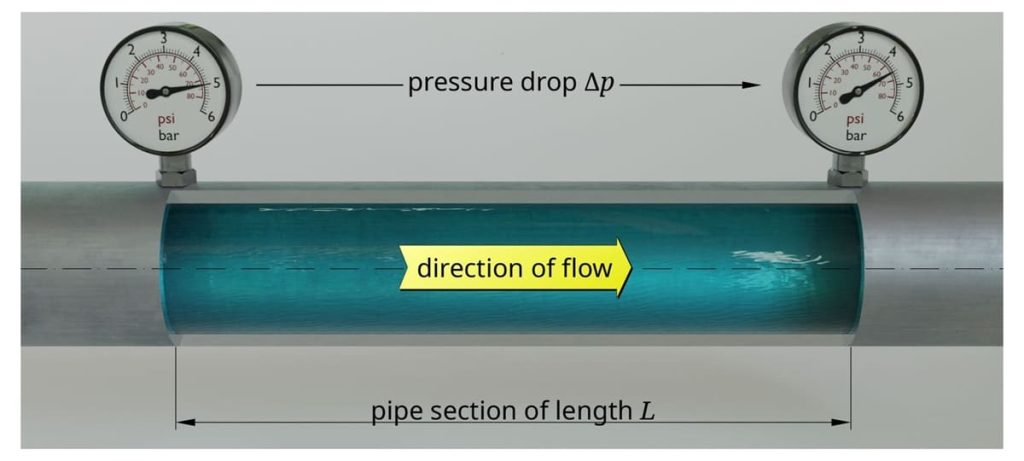
The calculation of head loss in pipe is among the most important aspects to ensure the efficiency of an industrial plant. The analysis of this phenomenon, determined by the reduction of fluid pressure flowing inside the pipe, is indeed essential to ensure the efficiency and operational safety of the plants.
Calculating head loss in pipe helps prevent inefficiencies, failures and malfunctions, ensuring proper sizing and optimal management of piping lines.
In this article, we will discover the head loss in pipe formula, analyzing the main variables, such as fluid viscosity, flow velocity, internal pipe diameter, and the roughness of their inner walls.
What is head loss in a pipe
Pipe head loss, or head loss, occurs due to various factors, such as internal fluid friction, turbulence generated by bends or restrictions, and resistance offered by various components of the plant, such as valves and fittings. The consequences of an incorrectly calculated head loss can be significant and can result in, for example, oversized pumps, excessive energy consumption, and deterioration of piping lines.
For this reason, industrial design software includes modules dedicated to calculating pipe head loss. Among the best solutions is ESApro Head Loss, which, starting from the three-dimensional model of the plant, calculates the total pipe head losses (of the analyzed section and each component) and verifies the correct sizing of the piping line. The software can automatically retrieve the components installed on the section, generate a spreadsheet with geometric data, and associate each component with its resistance coefficient.
Pipe head loss calculation is indeed essential during the design of a plant and is indispensable to ensure the efficient operation of multiple applications: examples include the piping lines of industrial plants, heating and cooling systems, hydraulic networks, irrigation systems, and water treatment. An accurate estimate of pipe head losses is also fundamental for the correct selection of pumps and components: it ensures that they are adequately sized to maintain the desired flow within the pipes.
How to calculate head loss in a pipe
This process involves the use of mathematical equations and fluid dynamics principles to determine the reduction of fluid pressure along the pipe path. The calculation methods vary based on the nature of the flow (laminar or turbulent), the characteristics of the fluid, and the specific configuration of the pipe.
Pipe head losses are therefore influenced by the fluid’s ability to flow through various components, such as valves and fittings. In this context, it is also useful to , the coefficient that provides a direct measure of how easily a fluid can pass through a valve: a higher value indicates greater ease of passage and therefore, in theory, lower pipe head losses.
We can distinguish two main types of pipe head loss, let’s discover them together.
Distributed head loss
They occur along the entire length of the pipe and are mainly caused by friction between the fluid and the inner walls of the conduit. Distributed pipe head losses depend on the length of the pipe, its diameter, flow velocity, internal roughness of the pipe, and the physical properties of the fluid, such as viscosity.
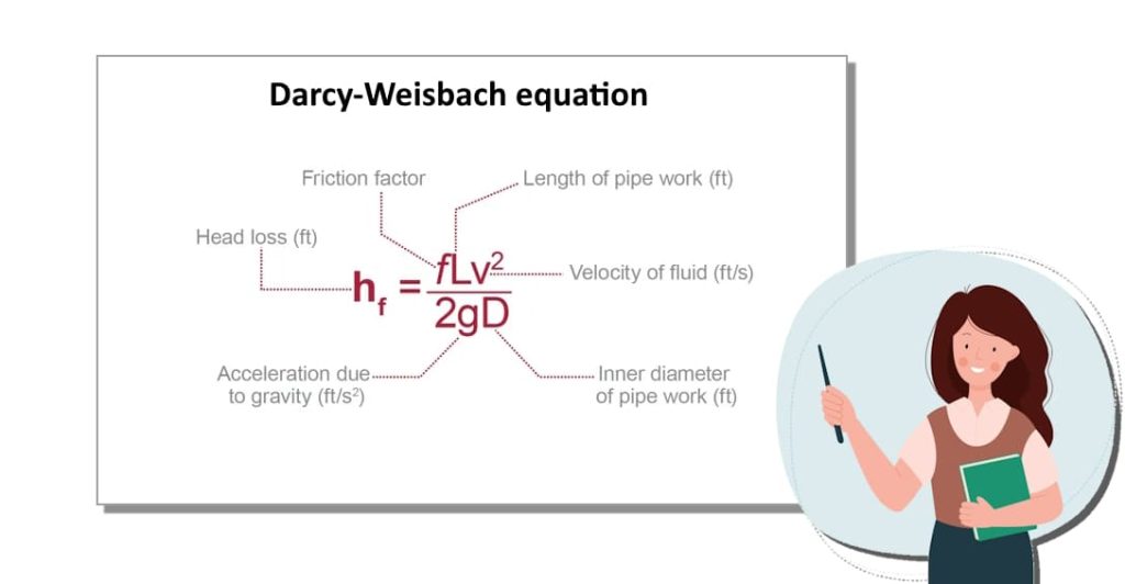
For the calculation, the Darcy-Weisbach equation is generally used, along with the determination of the friction factor, which can vary depending on the flow regime (laminar or turbulent).
Darcy-Weisbach equation Hf = f (L/D) x (v^2/2g)
Where:
- “f” is the friction factor
- “L” and “D” are the length and diameter of the pipe (m), respectively
- “v” is the fluid velocity (m/s)
- “g” is the acceleration due to gravity (expressed in m/s²)
Localised or concentrated pipe head loss
Localized or concentrated pipe head losses occur at specific points in the piping lines due to the presence of certain components, such as valves, bends, fittings, expansions, or restrictions. They are therefore independent of the pipe length and are associated with changes in the direction or velocity of the fluid, which cause turbulence and additional flow resistance.
To calculate them, specific loss coefficients for each component are used, which consider the extent of the disturbance that each element introduces into the fluid flow. At these points, the fluid undergoes a sudden change in direction and velocity due to friction and turbulence: this results in the conversion of pressure energy into thermal energy, leading to significant temperature increases.
To calculate them, we can use the following formula:
∆p = K ∙ p ∙ v2 2 ∙ 100 (bar)
Where:
- “K” is determined experimentally
- “p” is the fluid density (expressed in kg/dm³)
- “v” is its velocity before the deviation or restriction (m/s)